


Black Scholes Option Pricing Model
A Tutorial and Spreadsheet

A Quick Side Note
Before I get into the main topic of today’s newsletter, I want to comment on something that is an important issue related to economic development. There are essentially two ways to create economic growth:
Increase the supply of labor — get more people working
Increase the productivity of labor — either through investing more in capital (productive equipment) or through technological advancements.
Fortunately, these are not just arbitrary factors that are outside of our control. Instead, we influence these with economic policy. Things like job training programs, public education, tax codes that encourage investment, and regulations that make society operate more efficiently (such as traffic laws). After spending my first ten years or so in higher education, one thing that I noticed was the number of excellent students (hard workers, intelligent, ethical, etc.) that were not US citizens and, as a result, had a MUCH harder time staying in the US to establish their career regardless of whether or not they wanted to do so. These were potential members of the labor force who likely would be highly productive, help push forward economic growth, and likely pay quite a bit of taxes over their lifetime. In other words, the kind of people that any nation would be happy to have in the workforce and community. Unfortunately, many of them struggled to find employers that would work with their immigration status or were unable to establish citizenship without jumping through many complicated hoops.
So when I saw the following tweet from Mostly Borrowed Ideas (someone who is well worth a follow if you aren’t already doing so), I couldn’t help but nod my head in agreement. This is not a post recommending the removal of borders, just a thought that we should not work so hard to actively discourage people from joining, and powering, the US economic engine if we want to see the US economy operate at peak performance. Instead, actively encouraging productive folks to help power that engine forward and make it as efficient as possible seems like a much smarter idea!


The Black Scholes Option Pricing Model
If I had to list the ten biggest contributions to the field of finance, one that would be a clear shoo-in for inclusion would be the BS OPM. This is not because it is a perfect model (although, it does work amazingly well), but because it is a driver to one of the faster growing financial markets over the past few years.

Without the BS OPM, publicly traded options as we know them likely would not exist.1
Full disclosure in that I am NOT an options expert. While I have taught option basics to thousands of people and have traded options, I feel that for the vast majority of people, options fit Warren Buffett’s description of derivatives as weapons of mass destruction rather than sound investment tools.2 Options are essentially a zero-sum game (before taxes and transactions costs) and a negative-sum game with all costs realized.3 If you aren’t interested in options (which is a perfectly reasonable perspective), come back next week. With that disclaimer out of the way, let’s get this party started.
A Video Tutorial and the Spreadsheet
Here is the BS OPM spreadsheet. I put this together for teaching investments probably about 15 years ago or so. The reason for that is that the BS OPM is a relatively complex calculation and working through the calculations by hand each time is a bit of a nightmare. It is much easier to do it with the aid of computerized calculations. Note that you can even find online calculators pretty easily such as this one by GoodCalculators.com. My lack of programming skills and desire to get students familiar with Excel led me to the spreadsheet route.
To go with the spreadsheet, here is a “quick” video tutorial.4
Black Scholes Model
Here are a couple pdf files which you may find useful as you move through this week’s post.
The first provides a couple of examples that we will walk through and the second provides the actual model.
Let’s start with the definitions:
A CALL option is the right, but not the obligation, to buy the underlying stock for a fixed price within a specified time frame.
A PUT option is the right, but not the obligation, to sell the underlying stock for a fixed price within a specified time frame.
Each option contract is for 100 shares of the underlying stock and options typically expire weekly for the next several weeks, then monthly (on the 3rd Friday of the month) after that. Here you can see a list of upcoming Amazon options.

Most options are relatively short-term in nature (anywhere from a few days to a couple months). Each option contract requires two parties — someone to buy the contract and someone to write the contract. The option writer is obligated to take the other side if the option owner decides to exercise the option. The fixed price is referred to as the strike (or exercise) price.
There are five factors that determine the value of an option (note that all relationships use the ever-famous academic disclaimer of “all else equal”):
The price of the underlying stock. As the stock prices rises, this will increase the value of a call and lower the value of a put.
The strike (exercise) price. This does not change over the life of the option, but option buyers can choose which strike price they want to buy. For a call option, higher strike prices are cheaper and lower strike prices are more expensive. The opposite is true for put options.
The time to expiration. An option is essentially a side-bet on the movement of the underlying stock price. However, it is not a symmetrical side bet. If I buy a call option with a strike price of $70 per share, my option will expire worthless if the stock is below $70. It doesn’t matter if the stock trades at $69.88 or at $6.99, the option is going to be worth exactly $0 at expiration. However, the higher it goes above $70, the more I make. At expiration, if the stock is at $71, the option will have a value of $1 (or $100 for the contract). If the stock goes to $75, the option will have a value of $5. If the stock goes to $100, the option will have a value of $30. Therefore, the more time until expiration the greater the potential for the stock to move up OR down. But since the payoff is not symmetrical, bigger movements are better for the option owner. Therefore, the longer the time to expiration (for both calls and puts) the more the option will be worth.
The volatility of the underlying stock. The reasoning here is the same as time. A stock that may only move up or down by 1% in a good month or bad month is not going to create big swings. Alternatively, stocks that move 2% or more on an average day are going to create much bigger swings. The greater the volatility, the more potential for the asymmetric payoff pattern to work in my favor. Again, I don’t care if the stock closes at $69.88 or $6.99 with a $70 strike call, it is still worth $0. However, the difference between closing at $71 and $100 is huge.
The risk-free rate of interest. This is a bit more complex, but ties into the idea that I can create a risk-free position buy buying a put option contract, writing a call option contract (with the same strike and expiration as the put) and buying the underlying stock. Doing so will ALWAYS pay me the strike price at expiration. It doesn’t matter if the stock goes up or down, I have locked in the exercise price. However, I don’t get it until the options expire. Therefore, the cost of creating this position should equal the present value of the exercise price. We can estimate the risk-free rate by the Treasury bill rate matching the time to expiration for the option.
In the example pdf, you see the following information:
The time to expiration is 40 days. We input this as the number of years. Since there are 365 days in a year, this is 40/365 for time.5
Next we have the strike price at $60.
Then, the stock price at $62.
These are followed by the volatility of 32%. A couple of quick notes on volatility. This is the only one of the five variables we don’t know. We can use a calendar to count days, we select the strike price we want, we can easily see the stock price, and the risk-free rate is the Treasury bill rate. All of these are easy. However, the volatility should be how much volatility the stock will see on an annualized basis between now and expiration. Maybe your Magic 8 ball is more reliable than mine, but mine does a poor job of predicting the future. One way to estimate this is to see what it has been over the past 3-6 months and assume that it will be similar going forward. However, earnings announcements, CEO changes (hey, Twitter), etc. can cause spikes in volatility that should be factored in.6


And finally, we have the risk-free rate of 4% which we would just plug in.
Doing this would tell us that the call value is $3.86 while the put value is $1.60. Note that this does not say “it will cost $3.86 to buy the call and $1.60 to buy the put.” Instead, it says, “based on the model and our estimates, the value of the call is $3.86 and the value of the put is $1.60.” It is quite possible that our values could be off due to a poor estimate of volatility or due to some slight errors in the model.7 Therefore, if you have confidence in your estimates and the model and the call option is trading for $4.75, you would either (a) look for another option or (b) decide to write the option rather than buy it.
Intrinsic Value and Speculative Premium
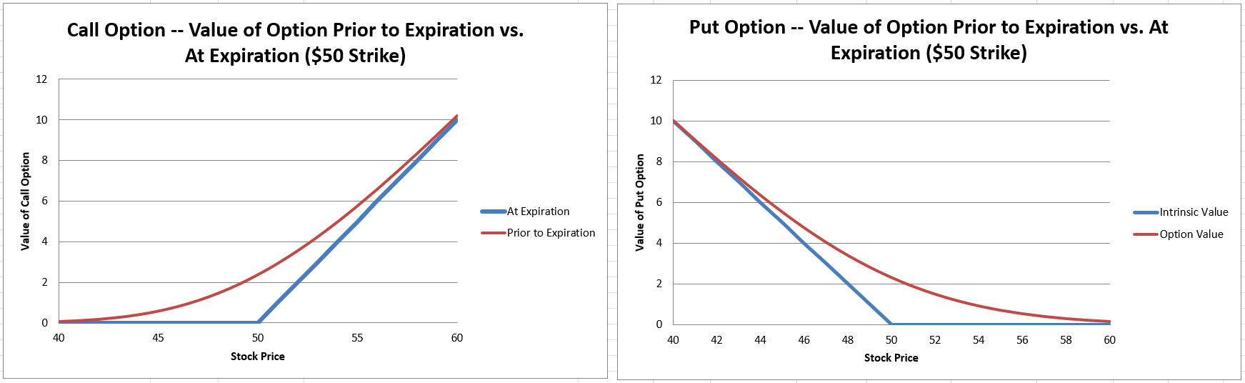
Option values can be split into two components. Intrinsic value (what the option would be worth if it expired right now) and speculative premium (the extra value the option provides due to its asymmetric payoff pattern). Therefore, the value of the options can be written as

Note that the intrinsic value can not be below zero. That is because you do not have to exercise your option. If it is going to cost you more to buy the stock using your option contract than the stock is worth, you’d simply let the stock option expire worthless. In our example, the stock was trading for $62 and the strike price was $60. Therefore, the intrinsic value of the call was $2.00 and the intrinsic value of the put was $0.00. However, in both cases, the VALUE of each option was higher than this ($3.86 for the call and $1.60 for the put). That is because with the option, the most we can lose is fixed, but the upside is much larger. This creates the speculative premium. Also, because the speculative premium will always be greater than zero, we will never exercise the option early (assuming no dividends) and would exit by selling in the secondary market rather than exercising. For instance, instead of exercising the call and getting $2.00, I could sell it to someone for $3.86…a much better deal. Essentially, your option value should appear as the red line on these graphs while the intrinsic value is the blue line. Note that the speculative premium will be largest when the stock price is essentially equal to the strike price. Then it will get smaller as the option drops further out-of-the-money (would expire worthless) or moves further into-the-money (would be exercised when it expired). This is because the further out-of-the-money the option falls, the bigger the movement necessary to bring the option back into value at expiration (so there will be a larger chance of it expiring worthless). Alternatively, the further in-the-money the option is, the greater your potential loss if the stock moves in the opposite direction.
It’s All Greek To Me
Another component of option valuation and strategy are the Greeks. These are measures of the option’s sensitivity to the key underlying variable. Even though there are five factors that drive the value of the option (time to expiration, the strike price, the stock price, the volatility of the underlying stock, and the risk-free rate of interest) and there are five Greeks, they do not line up exactly. That is because of the five factors driving the option values, one of them — the strike price — will not change while you own the option. Therefore, we don’t need to measure the sensitivity of the option to the strike price. Instead, we add a second measure of sensitivity to the underlying stock price (delta and gamma). You can see the breakdown in the following pdf.
These are discussed a bit in the tutorial video if you are interested, so I’m not going to spend time going through them here. When the meme stock craze hit the markets in early 2021 with GameStop and AMC, you may have heard the terms short squeeze and gamma squeeze. Here is a short article explaining the concept of a gamma squeeze.
Implied Volatility
Many retail options traders, especially those early in their options trading career, are probably buying options as directional bets on stocks. In other words, if I think the stock is going to rise, I can buy a call option. If I think the stock is going to fall, I can buy a put option. This will give me two advantages — less capital required and higher potential leverage. For example, right now Amazon is trading for about $3500 per share. Buying 10 shares will cost $35,000. However, a January 3500 call option which expires January 21st costs about $165. Therefore, I can control 100 shares of Amazon for $16,500 (less than half of what it would cost me to buy 10 shares). If Amazon climbs to $3800 by the option expiration, I make a profit of $135 per option (or $13,500 on the contract) and nearly double my money.
That said, option purchases are more about predicting volatility than price direction. This is not to say that you can’t make money trading options based on predicting the direction of the stock movement, just that volatility swings are what make options “cheap” or “expensive”. Volatility is also the only true unknown in the model as it is not past volatility we want, but future volatility. Fortunately, we can back out what the market is pricing into the model. This is referred to as implied volatility.
In the example, we have 30 days to expiration (30/365), a strike price of $55, the stock is trading for $53.50 and the risk-free rate of interest is 3%. Also, the call option is trading for $1.43 and the put is trading for $2.80. What we don’t know is the volatility that will make this work out. We can figure that out by plugging in a value. If I start with 30% for volatility, the option prices are too high. In order to make the BS OPM values increase, I need to increase volatility. By trying 35%, I now have overshot the prices. Therefore, the implied volatility is between 30% and 35%. Trial-and-error gets me to 33% for the implied volatility. If I think volatility is higher than 33%, then these options are too cheap and I should buy them. If I think volatility is less than 33%, then these options are too cheap and I should either look for a different trade or I could write the options.
Conclusion
This is getting pretty long. There are two more tabs which introduce spin buttons as a way to experiment with changing inputs into the model to show how that impacts option prices and speculative premiums, but I’ll let you look at the video if you are interested. If you have any questions, please don’t hesitate to leave a comment.
Note that the options pricing model would almost definitely still be here even if the guys who developed it never existed. Such is the nature of scientific development.
The specific quote is “In our view, however, derivatives are financial weapons of mass destruction, carrying dangers that, while now latent, are potentially lethal” and comes from the 2002 letter to shareholders.
Sorry for all the footnotes, but want to clarify this one a bit. An option is effectively a side-bet. The buyer of the option owns the right, but not the obligation, to buy the underlying stock for a fixed price within a set time frame. The writer of the option is obligated to deliver the underlying stock if the option owner decides to exercise. Therefore, every dollar made by the option owner is lost by the option writer or vice-versa. Any profit by the option owner is a loss to the option writer. Once we introduce taxes and transaction costs (bid-ask spreads, brokerage fees, time, etc.), options are effectively a negative sum game due to the “leaks” caused by taxes and and costs of trading. This does not mean options are a waste, there are some legitimate reasons to trade them. However, I would argue most trades are probably more akin to sports betting or casinos than investing (not that there’s anything wrong with that as long as you recognize the game you are playing).
Okay, it’s not really quick at over 35 minutes. Sorry, I understand the desire for short videos, but that is just not in my wheelhouse. If you choose to watch the video, feel free to pause and watch it in breaks.
Time is the number of years (usually, but not always, less than one). One question that comes up is whether to use t = (days remaining/days per year) or t = (trading days remaining/trading days per year). Because markets are closed on Saturdays, Sundays, and certain holidays, the trading days per year works out to 252 vs. 365 days per year. In practice, it won’t make much difference because the ratio should be similar. However, there are some arguments for short-dated options that days remaining/days per year is better.
Another issue is annualizing volatility because you are often estimating from daily or weekly returns. The way to do this is to multiply the observed volatility by the square root of the number of observations per year. Therefore, if I have weekly volatility as 1.5% and there are 52 weeks per year, my annualized volatility would be 1.5%*(52)^0.5 = 10.82%.
One cautionary note is that this model assumes non-dividend stocks. If your stock has a high dividend that would be paid between the time the option is established and when it expires, this could lead to a minor price error. There are also some issues with volatility smiles and/or volatility skew. That said, these errors will be relatively small.
Hi Kevin how can I contact you?