


A Quick Look at Returns
Behavioral Biases and Arithmetic vs. Geometric vs. Dollar-Weighted Returns

First, thanks to everyone who subscribed and helped promote my newsletter. The level of support is much appreciated. Please feel free to reach out (you can just leave comments here) with feedback or things you’d like to read about. Also, I hope everyone had a great 4th of July weekend!
Onto the topic for today…returns.
Here’s your TL;DR summary1
We do a poor job of understanding returns due to both behavioral biases such as overconfidence and optimism and because returns over time are trickier than we’d think at first glance.
Dollar-weighted returns >>> Geometric returns >>> Arithmetic returns.
Geometric average returns will always be lower than arithmetic average returns.
The more volatile the return stream, the more important it is to use dollar-weighted or geometric average returns.
A 50% loss is NOT offset by a 50% gain (it only gets us half of our money back) and a 75% loss requires a 300% gain to get back to even.
When saving for retirement, it is better to get our higher returns later in the savings period than early. This reverses when we are in retirement and it then becomes more valuable to get higher returns early in retirement.
There’s a joke in finance that a stock down 90% is a stock that was down 80%, before it got cut in half. In my previous post, I talked about one of the levers of compounding wealth being returns. However, the reality is that most of us do a poor job of understanding returns. This can be due to our own behavioral biases and because returns are tricky.
Let’s start with a couple of basic behavioral biases that are closely related – overconfidence and optimism. Overconfidence bias leads us to a subjective belief that our ability is greater than the objective reality of our ability. Optimism bias essentially allows us to ignore base rate and assume that our results will be far better. We can see both of these show up in an Allstate survey of driver behavior from 2011 where 64% of drivers rated themselves as either excellent or very good. As a side note, I would often do this in one of my classes and typically had about 70% or more students rate themselves as better than average drivers and only about 10% would be below average. Optimism bias shows up when we rate our close friends or other people our age. In the same survey, only 29% of close friends and 22% of other people their age were either excellent or very good. And out-of-state drivers? They should be banned from the roads as only 8% were excellent or very good. These are likely factors impacting US investors expected returns on their investments, which according to a recent survey were 17.5% above inflation! This seems…not good.

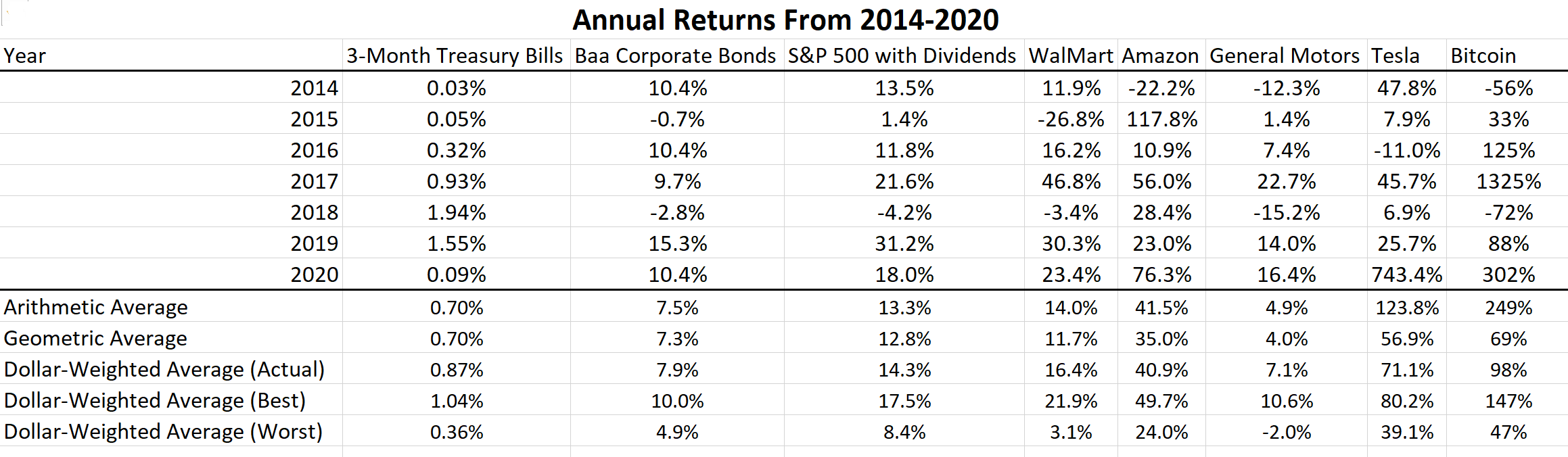
Now, back to returns. Often in finance when we are introducing compounding, we assume returns are constant from year to year, for example, what happens when I save $500 per month at 8% return for 20 years. Unfortunately, this is not reality. Returns vary, often dramatically, from year to year. Take a look at the following table:
When returns are not constant from one period to the next, both the volatility of the returns and the timing of the returns can impact how much our money will grow over time. There are three ways we can calculate returns – arithmetic average, geometric average, and dollar-weighted average. Unlike with classes, there is no test here, so you ignore the calculations and just think about the concepts.
Arithmetic average returns calculate averages the way most of us calculate averages. Add up the totals and divide by the number of observations. If I earn 7%, 10%, and 13%, my total is 30% and the average is 10%. The downside to this is that (and allow for some exaggeration here) if I earn 100% in year 1 and -50% in year 2, my arithmetic average is 25% per year. However, if I started with $1, it grew to $2 at the end of year 1 and then fell back down to $1 at the end of year 2. Clearly, my average return was not 25%.
Geometric averages are better as they take into account the power of compounding so that a 100% return followed by a 50% return would show a zero percent average return. The formula gets a bit messier (feel free to skip the math…again, there are no exams!), but it is essentially taking the nth root of the product of (1 + return) for each year. So, in our example, there are two years. The first year has a 100% return (which is expressed as 1.00 in decimal) and the second year has a -50% return (which is expressed as -0.50 in decimal). This gives us
[(1+1.00)(1+-0.50)]^(1/2) - 1 =
[(2)(0.5)]^(1/2) – 1 =
1 – 1 = 0%.
Dollar-weighted returns are the best measure of our return as they take into account how much money is invested at the time the returns are generated. Think about someone that saves $5000 per year at the start of the year for 5 years and gets 0% returns each year for the first 4 years and then gets 100% in the last year. That person will have FAR more wealth at the end of the 5-year period ($50,000) than if they earned 100% in year 1 followed by 0% returns each of the last 4 years ($30,000)2. In the first scenario, our investor earned just over 24% for their average return vs. only a little over 6% in the second scenario. To get the numbers in this table, I assumed $5000 invested at the start of each year for
the actual sequence of returns
the sequence with lowest-to-highest for the best returns
and the sequence with the highest-to-lowest for the worst returns.
As you can see, sequencing of returns matters quite a bit. I’ll come back to this in a future post.
At this point, you might be thinking “Silly academic types getting caught up in a lot of math. Does it really matter?” The answer, at least in this case, is yes. Surprisingly, sometimes these seemingly pointless distinctions DO matter in real life. To illustrate this, let’s go back to the table with 7 years of returns for a few different investments.
As you can see in this table, the 3-Month Treasury is pretty stable from one period to the next. This causes the arithmetic and geometric averages to be almost identical (the geometric average is technically lower by 0.26 basis points — 0.7014% vs. 0.6988%). The corporate bonds have a difference of about 20 basis points and the S&P 500 (stocks) are different by about 50 basis points. Once we get to individual stocks, the difference grows and Bitcoin is even more dramatic (6690 basis points and 18,000 basis points respectively). What this means is that the more stable returns are, the less relevant this difference is. The bigger the swings from year-to-year, the more relevant it is. For perspective, the difference in basis points for the S&P 500 from 1928 to 2020 is 185 basis points. Someone that would have invested $100 per year at the arithmetic average from the start at the 11.64% return would have $26,859,339. At the more realistic return of 9.79%, it would be $6,638,130…just a SLIGHT difference.
Remember the joke that started this post? A stock down 90% is a stock that was down 80%, before it got cut in half. Here’s the important take away. When you take a loss of 50% on an investment, that investment needs to double before you are back to even. What about when you lose 75% on an investment? Then the stock needs to double…and then double again (a 300% return) before you are back to even. The stock that lost 90%? A 100% return only gets you back to down 80%, the stock needs to go up by 900% in order for you to get back to even! This also works in reverse. If you quadrupled your money on an investment, a 75% loss wipes out all of your gains. Returns and losses do not offset each other on the same investment because the base shrinks when you lose money and grows when you make it.
When we look at dollar-weighted returns, this tells us that when we are saving for retirement, the returns over the first 5-10 years are not very important. It is the returns over the last 5-10 years that are critical to building wealth. This is because over the first several years, you probably haven’t accumulated enough wealth that it will be greatly impacted by the return. Over the last few years, you have all the savings you’ve accumulated up to that point in your life. A negative 20% return when you have $20,000 saved hurts, but it’s not really that relevant. However, a negative 20% return when you have $800,000 saved is MUCH more painful. Once you retire, the first several years of retirement are critical. Earn larger than expected positive returns and you build a big cushion. Earn less than expected, or even negative returns, and you not only are drawing out for living expense, but seeing your portfolio value shrink besides. These create “tipping points” where you may need to adjust your spending downwards in order to stay solvent or where you hit “escape velocity” and your account grows despite your planned spending.
There’s a lot more to returns, which I plan address over time, but this seems like a reasonable stopping point for today.
TL;DR = Too Long; Didn’t Read
In the first case, we’d have $5000(1 + 0.000) ==> ($5000 + $5000)(1 + 0.00) ==> ($10,000 + $5000)(1 + 0.00) ==> ($15,000 + $5000)(1 + 0.00) ==> ($20,000 + $5000)(1 + 1.00) ==> $50,000. In the second case, we’d have $5000(1 + 1.00) ==> ($10,000 + $5000)(1 + 0.00) ==> ($15,000 + $5000)(1 + 0.00) ==> ($20,000 + $5000)(1 + 0.00) ==> ($25,000 + $5000)(1 + 0.00) ==> $30,000.
Then to calculate the return:
Our PMT would be negative 5000
Our FV (in case 1) would be $50,000 (in case 2 it would be $30,000)
Our N would be 5
Our PV would be 0
And we’d solve for the rate of return.